Update
Steve McIntyre has taken exception to this post, with his own post entitled Sliming by Stokes. He has claimed in the comments here that:
"Stokes’ most recent post, entitled “What Steve McIntyre Won’t Show You Now”, contains a series of lies and fantasies, falsely claiming that I’ve been withholding MM05-EE analyses from readers in my recent fisking of ClimateBaller doctrines, falsely claiming that I’ve “said very little about this recon [MM05-EE] since it was published” and speculating that I’ve been concealing these results because they were “inconvenient”."
I've responded in a comment at CA giving chapter and verse on how he avoided telling the Congressional Committe to which he testified, which had a clear interest, about these inconvenient results. So far, no response (and of course no apology for the "sliming").
That was shown in MM05EE, their 2005 Paper titled:
"The M&M critique of the MBH98 Northern Hemisphere climate index: update and implications". I've shown that plot in an appendix here, and I'll show it again below. But for here, I'll show the plot with the MBH decentered and M&M centered superimposed.
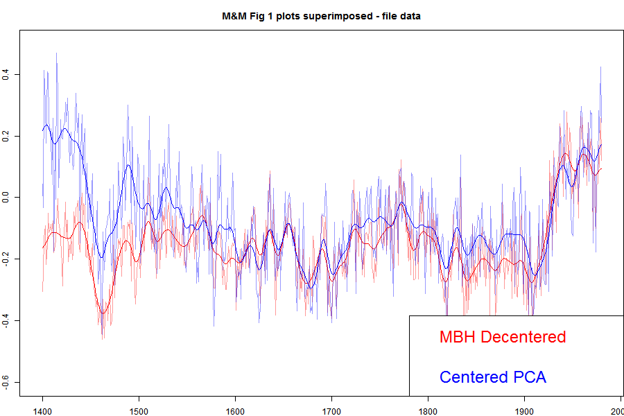
Update: When I printed out the data from my running of the MM05 code for Carrick below, I noticed discrepancies between the numbers and the emulation.txt data on file. I've tried to track down the reason, but I think the simplest thing to do is to switch to using the emulation.txt data directly, which I've done. The MBH and the corrected still track closely in recent centuries, but there is a somewhat larger discrepancy in the 19th century. Prvious versions are here and here..
The agreement is very good between, say, 1800 and 1980. These are the years when all the alleged mined hockey sticks should be showing up. They aren't. There is a discrepancy in the earlier years, which DeepClimate explains here. When Wahl and Ammann corrected various difference between the M&M emulation and MBH99 (in their case) this early period discrepancy disappeared. But anyway, for now what is important is that both centered and uncentered agree very well in the period where decentering is supposed to be mining for hockeysticks. Steve Mc has said very little about this recon since it was published, so much so that when Wegman was pressed (properly) by Rep Stupak at Congress on why he hadn't shown the results of a corrected calculation, he had no good answer, and didn't refer to M&M2005, even though he was supposed to be familiar with the code (which he had) which did it. I think this has become a very inconvenient graph.
I described earlier how apparent PC1 alignments have an effect on reconstruction that disappears rapidly as more than one PC are used. I'll give below a geometric explanation for this, which explains the irrelevance of MM)5 fig 2, which resurfaced as Wegman's fig 4.2.
Here is the plot direct from MM05EE. The bottom "centered" includes the removal by M&M of the Gaspe cedar data from 1400-1450, which affects those years.
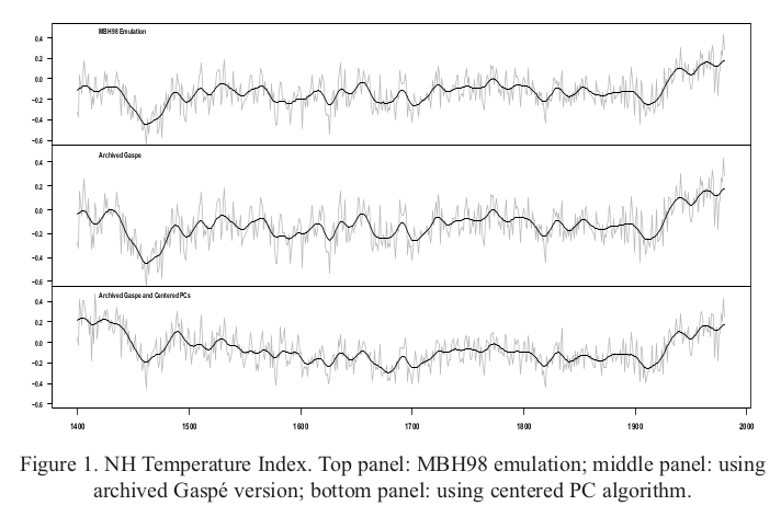
I've described the Gaspe issue, with some more plots here.
With trouble over the 100/1 sampling, Steve McIntyre has promoted his histogram, which appeared as Fig 2 in the MM2005 GRL paper, and as Fig 4.2 in the Wegman Report. The present re-presentation as a t-statistic adds nothing.
I've explained any times how all PCA is doing here is realigning the axes so that PC1 aligns with HS behaviour. In the simulated case, without that the axis directions are not strongly determined, and with white noise, not determined at all. That last means that all possible configurations are equivalent and would give the same results in any analysis. It takes only a slight pertuebation for one alignment to be preferred - how strongly depends on the randomness, not how much difference the alignment makes. I used the following analogy at CA:
Again there is no evidence that any aspect of Mann's decentered PCA has ever affected a temperature reconstruction, despite all the irrelevant graphics about PC1.
"Let me give a geometric analogy here. Suppose you live on a non-rotating spherical earth. You want a coordinate system to calc average temperature, say. You want that system to have a principal axis along the longest radius. You send out teams to measure. Their results have no preferred direction. There is a Pole star, so you histogram a Northness Index. It looks like the first one here. A sort of cos.
Now suppose the Earth is very slightly prolate, N-S, but the limit of measurement. Your teams will return results with a N-S bias. Your histogram of Northness will lbe bimodal like the second above. The spread will depend on how good the measuring is relative to the prolateness. If measurement is good, there will be rare few values, and the two peaks will be sharp.
The definiteness of the histogram has nothing to do with whether alignment of the principal axis matters."
Update. Here is the corresponding emulation from Ammann and Wahl. There is now no large discrepancy in the earleir years.
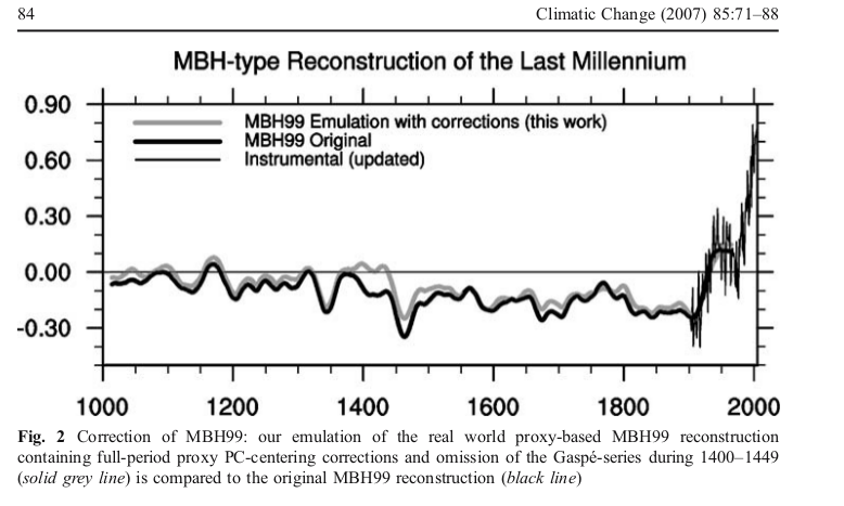
Update: DeepClimate, in a comment here, has linked to the plot below, which shows just how far MM2005 deviated from the MBH recon with centered mean - this time shown against the millenium recon.

Update: Pekka has added a comment which I reproduce with diagram below:
Pekka Pirilä October 8, 2014 at 9:00 AM
As this issue has been discussed so much, I wanted to understand it better and reproduced four variations of PCA of the NORAM1400 network:
1) short-centered MBH98
2) scaling as in MBH98, but fully centered
3) standard scaling and centering
4) without scaling of the original time series (MM05)
Otherwise the results are as reported elsewhere (e.g. in Wahl and Ammann, 2007), but I added the comparison of, how much each PCA explains by up to 10 first PCs calculating the shares from the real variability of time series used in each analysis. Thus the shares are calculated from the same total variance in cases (1) and (2), from slightly different in (3) and from substantively different in (4) where the variances of individual time series vary greatly.
The results are shown here

What many may find surprising is that my numbers for MBH98 are very different from those shown in several places (e.g. RealClimate). The reason is that those numbers are not based on the variability of the time series, but on variances around the short-centered mean. That adds both to the total variance and to the contributions from individual PCs. In relative terms it adds much more to PC1 than to the total. Thus the resulting number does not tell about the real variability, but is very much affected by the decentering.
I calculated my values by first orthonormalizing the basis relative to deviations from full mean (the mean affects, what's orthogonal), and by using this orthonormal basis for determining, how much the space spanned by N first PCs of the MBH98 analysis can explain.


No LIA. That is M+M's finding. Was few proxies in the 20th century in Marcot a problem for McIntyre? Why should it not be å problem for him in the 15th century?
ReplyDeleteWell, it's not really their finding - it's their rendering of the MBH finding, with centered PCA.
DeleteThere are reasons for the variance in 15th Cen, but yes, few proxies is certainly part of it.
What you seem to be saying is that McIntyre has falsely claimed that the MM PCA methodology selects hockeysticks whereas you are claiming that the MM PCA methodology produces the hockeystick directly by decentering.
ReplyDeleteIs this a fair.summary of your position? If not what are you claiming?
FC,
DeleteSelects what for? That's what everyone glosses over. MM say that short-centering selects (actually alighs) PC1 with hockey stick shape. Do you know what PC1 is?
I say that yes, it does, but that has virtually no effect on the subsequent reconstruction. And I think MM's graph shows that very well.
ATTP,
ReplyDeleteThat result is specific to the ITRDB data set used. I don't think it would be true for synthetic data for which a histogram could be prepared. In the synthetic, there is no specific HS cause, the short-centering tends to gather it as a pattern from random variation in a number of lower PCs. In the ITRDB it is real, and it is also found in centered PCA, where it appears as #4.
Nick,
ReplyDeleteI see. Let me see if I'm starting to understand this. If you did a full reconstruction using short-centered or standard centered, you would get roughly the same result. Therefore if you did a histogram of HSI for full reconstructions (rather than just for individual PCs) the histogram shouldn't depend on whether the method was short-centered or not. What you seem to be suggesting, though, is that the standard centered does not gather any particular signal when data is synthetic (presumably because it is spread across a number of PCs) and hence comparing histograms of individual PCs may not be particularly illustrative?
ATTP,
ReplyDeleteYes. The natural question would be - if it's random, why would any particular PC show out.
On recons, here is a very artificial example. Suppose you had that prolate earth, and a whole lot of different reference frames from different surveys. You decided to work out the average surface wind speed. The reference frames vary, but tend N-S.
So if you retain 1 PC, it will model mostly an average N-S component, and the histogram would show it (bias). If you retain 2, you'll get a much fairer representation. And if you retain 3, it should work perfectly, and a histogram would be physical.
Given the extremely long persistence in the synthetic data MM05 used, longer term departures (i.e. trends) should be expected, and given that the MBH98 methods find a hockey-stick PC1 in the synthetic data I rather expect that the MM methods will show a hockey-stick of some nature in one of their significant PCs.
ReplyDeleteFor the actual proxy data the MM05 hockey-stick was PC4,with PCs 3, 4, and 5 erroneously dropped due to not checking significance as per MBH. I haven't run the MM methods on their synthetic data to examine the principal components there, but I would be quite surprised if there wasn't one with a strong HS trend, and which would show a similar HSI histogram to the MM05 Fig. 2 MBH results.
In short, the centering convention used by MM05 shifts any hockey-stick trends to a different PC (and rather diffused by variance being spread across 5 PCs rather than 2), meaning that the Fig. 2 comparison of MBH PC1 should be tested against _all_ the MM05 PCs to be correct.
Good work Nick. Thank you for separating the chaff (McIntyre and McKitrick) from the wheat, and for keeping our eyes on the pea. McIntyre seems to be trying to bury his gross errors under a mountain of indignant blog posts, obfuscation and red herrings. McIntyre ought to just come clean, climb down and be honest with himself and others. That he can't do that, just goes to show how far gone and deluded he is. Sad really.
ReplyDeleteHe and Ross are having a tough week. KR at ATTP's place linked to a not flattering dissection of another weak attempt at statistics by McKitrick that he got published in a dodgy vanity journal.
You're out Nick.
ReplyDeleteNick,
ReplyDeleteYou say " MM)5 fig 2, which resurfaced as Wegman's fig 4.2." and then discuss "trouble over the 100/1 sampling". McIntyre said only days ago "The relevant MM05 figure, Figure 2, is based on all 10,000 simulations."
You are active in the CA threads where this is being discussed. Did you miss this statement, and if so will you correct your text?
I said at CA
Delete"Re
[Steve]“Stokes knows that this is untrue, as he has replicated MM05 simulations from the script that we placed online and knows that Figure 2 is based on all the simulations;”
[Me]I said at the start of my original post
“I should first point out that Fig 4.2 is not affected by the selection, and oneuniverse correctly points out that his simulations, which do not make the HS index selection, return essentially the same results. He also argues that these are the most informative, which may well be true, although the thing plotted, HS index, is not intuitive. It was the HS-like profiles in Figs 4.1 and 4.4 that attracted attention.”"
The fact that one plot does not use the selection does not make the other occurrences OK.
Anonymous writes: You are active in the CA threads where this is being discussed. Did you miss this statement, and if so will you correct your text?
DeleteYou presumably came here from CA, without reading the relevant thread here. MM Figure 2 is *not* the problem that Nick is discussing, and Nick made that abundantly clear.
McIntyre is acting like a driver who got ticketed for speeding and is now complaining to the judge that the officer was totally wrong because some other time he was staying safely under the limit. Sorry, but no.
The point here is the "sample" of 100 time-series that were published in the SI with MM05, and then turned into Wegman's figure 4.4. That "sample" of 100 series was highly un-representative. In fact, McIntyre's code weeded out the 99% of series that were least hockey-stickish, keeping only the 1% that most closely agreed with the point he was trying to make.
Nowhere in MM05 was this explained -- you need to work through the code to discover it.
Wegman saw the reference to a "sample" from the 10,000 random series" and thought (reasonably, IMHO) that it meant a "representative sample", though MM had carefully avoided labeling it as such. In reality, it was a massively biased sample. Wegman was misled by McIntyre, and the US Congress was misled by Wegman.
Now McIntyre is misleading you about what Nick has and hasn't said. My opinion of SM's reliability is dropping daily.
Ned W
Ned,
DeleteMy opinion of Nick's reliability is dropping just as fast. Nick claims that Fig 2 in MM05 "resurfaced" as Wegman's chart, in other words that it same as the Wegman chart. It cannot have "resurfaced" if Wegman used a different selection of data.
If Wegman's chart is the same as a chart in the SI of MM05, then it is up to Nick to say so and to correct his text above. If M&M's SI is so important, it is up to Nick to explain why, and not refer to a chart in the main paper.
Anon,
DeleteThe caption to Fig 4.2 in the Wegman report begins:
"Figure 4.2: This is our recomputation of the Figure 2 in McIntyre and McKitrick
(2005b).
"
Nick
DeleteThat may be what Wegman stated, but you know that it is not factually correct and that M&M used all 10,000 samples in their Fig 2.
I admire your ability to ask awkward questions and point out issues that are inconvenient to most readers at sites like CA. However your inability to correct even minor errors such as this one, and teh one about hosking.sim being "the blackest of boxes" (despite being only 23 lines of open source code with a book documenting it) really damages your credibility. In the scheme of things these are both minor points but for some strage reason you resist conceding them.
Anon,
Delete"n the scheme of things these are both minor points but for some strage reason you resist conceding them."
I resist conceding to what isn't true. I believe that both Wegman and M&M used all 10000. They could hardly have done otherwise. I referred to my statement about Wegman at the start of this subthread. I really can't see here what you want me to concede.
OK I withdraw that concern, but the one about hosking.sim remains, and perhaps you shoudl correct Ned who thinks that Wegman used a sample of 100 time series.
DeleteCan you please explain what you meant in your post, when you said "With trouble over the 100/1 sampling, Steve McIntyre has promoted his histogram," What trouble does SM have about 100/1 sampling? If this has been explained elsewhere, please let me know where to look as I've come to this discussion via CA rather than earlier posts of yours.
Anon,
DeleteThis post from a week or so ago is the start of the current series. It refers to other posts in 2010 and 2011. Basically, some much-promoted graphs in the Wegman report showed what were presented as typical cases, but there was an unstated step in which a batch of the 100 most HS-like of 10000 were selected, and then sampled for display. This was done in SM's code, and the batch of 100 that W used was in fact supplied by Steve.
So Wegman used code that was created by M&M. Did M&M actually use the selection in their paper, or was that just Wegman? If they didn't. it seems difficult to justify your claim that SM has "trouble over the 100/1 sampling" - though maybe Wegman does.
DeleteAnon,
Delete"Did M&M actually use the selection in their paper"
Yes, but less so than Wegman, because they did not show Fig 4.4, although the mechanics to create it are in the code. Their Fig 1, captioned "Top: Sample PC1 from Monte Carlo simulation using the procedure described in text applying MBH98 data transformation to persistent trendless red noise; "
was #71 in their archived selected 100. And they placed that 100 on the SI, described thus:
"Computer scripts used to generate simulations, figures and statistics, together with a sample of 100 simulated ‘‘hockey sticks’’ and other supplementary information, are provided in the auxiliary material "
"So Wegman used code that was created by M&M"
Not just the code, but the numbers. Both his 4.1 and 4.4 have curves that are not randomly generated, but taken from that selected archive.
Thanks Nick
DeleteThe comments on the post you linked to seem to be informative about the issue. I'm still not clear whether M&M did more than poorly label their SI code and numbers - which it then appears Wegman mis-used
Anonymous, 10:57pm:
Deleteperhaps you shoudl correct Ned who thinks that Wegman used a sample of 100 time series.
To be crystal clear about what happened here:
(1) M&M used a random process to generate 10,000 time series. Those 10,000 were the basis of the histogram in MM05 figure 2. Nobody is questioning that.
(2) M&M then wrote code to weed through the 10,000 series and pull out only the 1% that were most hockey-stickish in appearance. Those 100 were posted with the Supplementary Information on the journal's website. There was no explanation of the fact that this was a very highly biased sample (only the top 1%!) in either the paper or the README file with the SI. You can only figure it out if you work through the code.
(3) Wegman then used this "sample" as the basis for his Figure 4.4, on the mistaken belief that it was a representative sample.
OK, so far? That's the past. Now for the present:
(4) Nick and other commenters here point out that the process used to select the 100 time-series used in the SI for MM05 was strongly biased, and that the lack of any mention of this was problematic. (It obviously was misleading because Wegman, for one, was misled, and others who downloaded the 100 series from the journal's website may also have mistakenly believed they were a "representative sample")
(5) McI posts a thread over at CA trying to shift the subject to Figure 2, which no one here had claimed was based on just the cherry-picked 100. Nick (and everyone else over here) has always been clear that *Figure 2* was based on all 10,000 series. What we were discussing was Wegman's *Figure 4.4* and the MM05 archived set of 100 series that were the basis for it.
(6) People dutifully troop over here from CA and accuse Nick of being wrong about MM05 Figure 2, because McIntyre told them Nick was talking about MM05 Figure 2.
Anonymous, 11:58 pm:
I'm still not clear whether M&M did more than poorly label their SI code and numbers - which it then appears Wegman mis-used
That is the problem. MM05 didn't mention (outside the actual code) that the "sample" of 100 series was the result of a selection process that weeded out everything except the 1% that most closely confirmed their point. Then Wegman used the 100 series as the basis for Figure 4.4, under the (reasonable) impression that what MM05 coyly described as "a sample" was in fact a representative sample rather than an extreme cherry-pick. If Wegman made that mistake, it's likely that others did as well (including, er, ... me ...)
The further problem is that rather than just admitting that he should have handled this differently in MM05 and moving on, McI is now busy misleading his CA readers about the nature of the dispute.
Ned W
Nicely summarized.
DeleteThanks Ned. Based on your description, the bottom line seems to be that M&M did not describe accurately the sample in their SI, and if correct SM should certainly acknowledge this point. However the sample was not used in MM05 so this issue does not apply to the paper itself.
DeleteIt appears Wegman relied on his data for chart 4.4. Whether this chart is really significant I don't know, but it appears SM should also apologise to Wegman.
Whether this issue has any contemporary relevance is also unclear. It doesn't make MBH98 any less "wrong" and it doesn't remove Steyn et al's reasonable use of Wegman to doubt Mann's hockey stick.
While I haven't been following the Steyn's trial with any interest, I doubt that Steyn is being sued for expressing "doubt." Color me skeptical of your narrative framing.
DeleteBecause he is a "public figure", for Mann to win he has to show the defendents acted with "malice" - which is a legal term that broadly means that Steyn and the other defendents knews what they were saying was wrong, but went ahead and said it anyway.
Delete"it doesn't remove Steyn et al's reasonable use of Wegman to doubt Mann's hockey stick"
DeleteCalling Mann "Dr. Fraudpants", as Steyn did publicly just a couple of days ago, isn't simply expressing "doubt".
"....and if correct SM should certainly acknowledge this point." FYI, this point has been acknowledged.
DeleteDhogaza
DeleteAs you are no doubt aware, Steyn started calling Mann Dr Fraudpants after Mann claimed *in his court submissions* exonerations by studies that did not mention or investigate him even though his own book stated he was not the subject of one of the investigations, and after Mann claimed he had "absolutely nothing to do" with the WMO99 cover despite claiming credit for it on his CV. Steyn's amicus brief repeats the word "fraud" in respect to these false claims, and the CEI lawyers go so far as to say that Mann's lawyers should be censured for making false claims in court proceedings
"Mann claimed he had "absolutely nothing to do" with the WMO99 cover despite claiming credit for it on his CV."
DeleteThis is untrue, Mann made no such claim.
I mentioned this in the other thread, but McKitrick used selections from the "cherry-picked 100" in his "What is the Hockey Stick Debate About" explainer from 2005. There is no explanation that these were from the top 1% and implies that such results were typical.
Deletei.e. "In 10,000 repetitions on groups of red noise, we found that a conventional PC algorithm almost never yielded a hockeystick shaped PC1, but the Mann algorithm yielded a pronounced hockey stick-shaped PC1 over 99%of the time." [...] "In Figure 7, seven of the panels show the PC1 from feeding red noise series into Mann’s program. One of the panels is the MBH98 hockeystick graph (pre-1980 proxy portion). See if you can tell which is which."
http://www.uoguelph.ca/~rmckitri/research/McKitrick-hockeystick.pdf.
CCE,
DeleteThere's some interesting history there, which I should look into. In their Comment in Nature, 2004, they described a simulation of which they said:
"Ten simulations were carried out and a hockey stick shape was observed in every simulation."
That's not very quantitative; I'm surprised Nature allowed it at all, but I'm sure referees would want to see the evidence. I suspect they saw the first version of Fig 4.4. They describe it as if they did just ten runs. The later paper for GRL was first submitted to Nature. Ross McKitrick comments on that here, mentioning that the referee was impressed by:
"MBH seem to be too dismissive of MM’s red noise simulations. Even if red noise is not the best model for the series, they should have reservations about a procedure that gives the ‘hockey stick’ shape for all 10 simulations, when such a shape would not be expected."
So again, it seems that he has seen that tableau of 10. Whether it was at that stage filtered, I don't know.
Phil,
DeleteI'm not sure what you are denying when you say Mann made "no such claim", but in any case you are wrong:
In his court submission Mann wrote:
"The "misleading" comment made in this report had absolutely nothing to do with Dr. Mann, or with any graph prepared by him. Rather, the report's comment was directed at an overly simplified and artistic depiction of the hockey stick that was reproduced on the frontispiece of the World Meteorological Organization's Statement on the Status of the Global Climate in 1999"
Mann's CV states:
"Jones, P.D., Briffa, K.R., Osborn, T.J., Mann, M.E., Bradley, R.S., Hughes, M.K., Cover Figure for World Meteorological Organization (WMO) 50th Year Anniversary Publication: Temperature changes over the last Millennium, 2000."
Which do you believe: Mann's CV or Mann's court submission?
" Stokes’ most recent post, entitled “What Steve McIntyre Won’t Show You Now”, contains a series of lies and fantasies, falsely claiming that I’ve been withholding MM05-EE analyses from readers in my recent fisking of ClimateBaller doctrines, falsely claiming that I’ve “said very little about thults because they were “inconvenient”. "
ReplyDeleteCorrection
DeleteStokes’ most recent post, entitled “What Steve McIntyre Won’t Show You Now”, contains a series of lies and fantasies, falsely claiming that I’ve been withholding MM05-EE analyses from readers in my recent fisking of ClimateBaller doctrines, falsely claiming that I’ve “said very little about this recon [MM05-EE] since it was published” and speculating that I’ve been concealing these results because they were “inconvenient”.
I see that you have posted on this and I have replied.
DeleteI am not big on enforcing blog policies, but one thing I do encourage is that if you want to speak of lies, you should be specific. Say what they are and why you claim they are lies.
The person who posted above beginning "Stokes most recent post..." was quoting from the introduction of the latest post at CA
Deletehttp://climateaudit.org/2014/10/01/sliming-by-stokes/
Having just read the blog and 29 comments I find myself somewhat confused. When the term PC1 is used, from what data does this principal component arise? Is it known exactly where the original series of a number of climate related observations are, and are they still there? How does this PC1 relate to the PCs that Prof Mann included in the 112 series, of up to 593 rows, that I have believed led him directly to the HS plot?
ReplyDeleteWhen I looked at the group of published PCs in the 112*593 matrix - now a long time ago - I found that they were not totally uncorrelated. This puzzled me. I have the aforementioned data matrix, and have done a considerable amount of work on it, using simple straightforward methods, but would welcome some more information about this data set, in case I am labouring under a misapprehension.
Robin - a first time poster here
Robin, in this group of posts, the PC1 is being pulled from autocorrelated noise. Randomly generated pretend proxies.
DeleteNomenclature: there might well be less confusion if PCn were sub scripted with MBH. or MM.
ReplyDeleteHow about "C" or "S"?
DeleteM&M didn't invent centered PCA.
The notion of "sample" might also deserves due diligence:
ReplyDelete> In statistics and quantitative research methodology, a data sample is a set of data collected and/or selected from a statistical population by a defined procedure.
http://en.m.wikipedia.org/wiki/Sample_(statistics)
It might be interesting to find a run within the centered PCA similar to MM05b's fig. 1.
> and of course no apology for the "sliming"
ReplyDeleteSliming was just the word of the day, Nick:
> I can’t imagine that it was very easy for him to face up to these mistakes, but it’s a far better practice than trying to tough it out by sliming his critics [...]
http://climateaudit.org/2014/10/01/revisions-to-pages2k-arctic/
The Auditor is a fierce ClimateBall (tm) player.
Nick,
ReplyDeleteMcIntyre/Persaud has boasted in the past in public about correcting his errors. Can't recall if he said promptly though, so we may have to wait a while, likely a long while.
Hearing McIntyre/Persaud whine and lament about people supposedly "sliming" him is hilarious-- first, because it is false and second because sliming and defaming certain climate scientists is his entire purpose in life for God's sakes. Quick, get the poor chap a mirror!
McIntyre/Persaud is trying to use the old gambit of "offense is the best defense". Also you have the poor chap against the ropes and he is flailing, hence the juvenile silliness from him. It is well beyond pathetic for him at this point, he is nothing but an old angry and bitter man with a blog. Think about it, his holy grail crumbling in beautiful slow motion for everyone to see.
Egotistical maniacs like McIntyre/Persaud don't deserve the attention your giving them, but it does serve the important purpose of exposing their misdirection, distortion and dishonesty. So I'm all for it, keep up the good work. Hopefully none of Steve's acolytes (that he has all fired up with his rhetoric and deception and venom) won't start behaving badly.
Nick, would you henceforth delete all posts by "anonymous" of which seem to be several.
ReplyDeleteIt is trivial to enter a pseudonym, but this kind of conversation becomes hard to follow.
Ideally, there would be some way to change the menu to elimination the "Anponymous" abomination.
A pseudonym is jsut as anonymous ,without the confusion.
John,
DeleteI agree that it is trivial, but for some reason, people don't. Eli and Sou have standing appeals to not anon, and I'll have to do that. But I'm very reluctant to delete.
An occasional reminder would probably suffice, especially for new readers.
DeleteI claim credit for some of the anons above. My reason was simply ignorance of the features available on this site. I'm reluctant to create yet another login so chose anon as an easy option. Having just spotted the name feature as a result of this comment, I will use that in future
It's a shame that blogging software doesn't handle this.
DeleteA minimalistic approach might be to generate a numbered pseudonym (AnonXXX?) based on a one-way hash of the unsigned posters IP address - that would at least provide identifiable continuity for comments from the same machine. But I don't know of anyone who's implemented anything like this.
2005.01.27 Backgrounder for McIntyre and McKitrick “Hockey Stick Project”. This was infinitely more important than the paper, which very few non-experts read, but was useful for the press.
ReplyDelete"Our research shows fundamental flaws in the “hockey stick graph” used by the Intergovernmental Panel on Climate Change (IPCC) to argue that the 1990s were the warmest decade of the millennium. The original hockey stick study was published by Michael Mann of the University of Virginia and his coauthors Raymond Bradley and Malcolm Hughes. The main error affects a step called principal component analysis (PCA). We showed that the PCA method as used by Mann et al. effectively mines a data set for hockey stick patterns. Even from meaningless random data (red noise), it nearly always produces a hockey stick."
"In over 99% of the cases it produced hockey stick shaped PC1 series. The figure below shows 3 simulated PC1s and the MBH98 reconstruction: can you pick out the reconstruction?"
So, they show 3 of their PC1s in panel with MBH reconstruction, strongly implying equivalence. Of course all 3 PO1s are HockeyStickUp.
2005.04.04 What is The Hockey Stick About? McKitrick talk.
NOTE: that's the original version, a few errors were fixed later.
This contains false citations, cherry-picks, use of obsolete sources, low-quality sources, such that M&M were at best seriously incompetent scholars, especially given the curiosity that the errors consistently helped support their claims.
p.11 "The Mann algorithm efficiently looks for those kinds of series and flags them for maximum weighting. It concludes that a hockey stick is the dominant pattern even in pure noise."
"Figure 7. Seven panels are PC1’s from red noise data fed into MBH98 algorithm. One panel is the MBH98 hockey stick itself.
Again, this is M&M's PC1s compared to the real recon. Only HockeyStickUps are shown.
2005.05.11 The Hockey Stick Debate - Lessons n Disclosure and Due Diligence This was presented in Washington DC for think tanks CEI and GMI and is the "blueprint" for the Wegman Report.
This contains false citations, cherry-picks, use of obsolete sources, low-quality sources, such that M&M were at best seriously incompetent scholars, especially given the curiosity that the errors consistently helped support their claims.
p.18 '"Detects hockey sticks as dominant patterns (PC#1) even in red noise' + same 4 graphs as above, i.e., it compares their PC$1 with MBH recon.
A few years later, GMI put up an annotated, transcripted version of that talk.
Now you can see what they told the audience, PDF p.13-15:
"To show how strong this effect was, we wrote a paper published not long ago in Geophysical Research Letters where we fed a type of random numbers called “red noise” into the program and we showed that it reliably produces a hockey stick-shaped first principal component, even when there is no trend in the underlying process. It is just a curious thing."
(4 graphs)
"Figure 7 shows four graphs. Three of them are examples of “red noise” yielding hockey sticks from the Mann algorithm and one of them is the actual proxy data portion of their temperature reconstruction. If you have trouble telling which is which, that is the trouble."
Again they were all HockeyStickUps.
Well, put in an appeal: you can guess who bugged Eli and Sou to put in their appeals, which of course people still ignore, especially at Eli's, which means I've stopped reading a lot of threads there.
ReplyDeleteSo, think about some way to discourage the practice. Maybe a warning after an anon comment?
It's sad that blogging software is still so weak, at the very least there should be an easy borehole-equivalent less than deletion.
In practice, I'd suggest that if you said you'd delete, and then started doing it, suddenly there would be very few anonymous comments.
Nick, could you provide the time series for this analysis (first curve)?
ReplyDeleteYour blue curve looks to have more low-frequency variance than the red one does (loss of low frequency variance using the short-centered PCA is the issue vhere). There's an objective way of checking.
Carrick,
Deletehere is a comment from Brandon, in which he plotted the numbers from a file of Steve's and got similar results. My numbers should be identical. You might like to try the file that BS links, as a check. I'm happy to print out my numbers if there is a discrepancy.
Thanks Nick. I did a first pass on that data set. As I guessed there is an enhancement of low-frequency energy, though the effect isn't huge.
DeleteThis an average of the amplitude for periods > 200-years.
Also I'm skipping the final 80-years, as that is locked in by the regression analysis.
SERIES LF Enhancement re/emulation [dB]
MBH98 0.0
emulation 0.0
Gaspe.only 0.1
NOAMER.only 2.5
corrected 2.8
It occurred to me that some people may not be used to reading dB scale. So here's the series converted in to percent enhancment in low frequency scale.
DeleteSERIES LF Enhancement re/emulation [Percent]
MBH98 0.2
emulation 0.0
Gaspe.only 1.1
NOAMER.only 33.4
corrected 37.8
So not huge, but not negligible.
Carrick,
Deleteyour headings aren't clear. here's my interpretation:
MBH98 - mann's original
emulation - MM05 emulation of Mann as is
Gaspe only - above with Gaspe removed 1400-1450
NOAMER - similar
corrected - probably MM05 centered and with Gaspe and NOAMER removed.
If so, it seems NOAMER is making the difference
Carrick,
DeleteI remember now that the headings were those on the file. That doesn't make them any clearer, but does mean I can look them up.
Nick, I interpreted the columns the way you did. But if you post your version of the series, I'd be interested in analyzing them too.
DeleteOne issue I noticed is there isn't good high-frequency agreement between MBH 98 and M&M emulation (M&M emulation has more high-frequency noise). That probably doesn't matter for the sensitivity testing, but it is curious.
Answering my own q, I've looked at the code, and it seems surmaise was correct, except the last seems tot to have NOAMER removed. Carrick's reult certainly suggests that it has N removed, though, so I'll check that.
DeleteCarrick,
DeleteMy version is here. The numbers don't match that CA file exactly, not even the MBH data. Not sure why - I think I looked into this once before.
Nick Stokes, Carrick, the reason I got results similar to Nick Stokes is I miskeyed an index when plotting my graphs. I had opened two different files for the MM05EE paper. One had an extra column.When I plotted my graphs, I thought I had loaded one file but had actually loaded the other.
DeleteIncidentally, I'm curious why the MBH column in Stokes's file is different from the emulation column in Steve McIntyre's. McIntyre's matches the results provided by Michael Mann. If the MBH column is meant as MBH's results, there's no reason it should be different. If it is meant as an emulation of MBH's results, it's strange it would be so different when McIntyre's is not.
Brandon,
DeleteYes, I'm curious too, and I'm checking. I am of course using the MM05 code. The MBH is read in from a binary, not from the file, but as far as I can see it is the same as the file. For some reason the MBH data goes to the NHbeta() function prior to plotting (that's in the original); not sure what happens there.
I might revert to just plotting from the file.
I've tried to track down the reasons for the discrepancy, but there is a lot of data used, so I think the simplest thing to do is to plot directly from the emulation.txt file. According to the comments, the MBH column and the "corrected" column should correspond to panels 1 and 3 of the MM05EE Fig 1. The smoothed curves are somewhat different but track to about the same extent, except for some divergence late 19th century. I'm still somewhat curious whether the "corrected" here includes the NOAMER adjustment, as Carrick's result suggests, but I can't see from the code why it would.
Delete"For some reason the MBH data goes to the NHbeta()"
DeleteThat came out a bit muddled. The MBH version plotted by the code is actually the emulated version out of NHbeta(), not the file data. They are supposed to correspond, but apparently now do not. I don't think I've changed anything.
There's more information in Fig 3 of this CA post, reproduced by Steve in his response.nel on the left looks like the one now shown here, reproduced from file. The one on the right shows the effect of various modifications to align with Wahl and Ammann. The use of correlation PC's as in MBH rather than covariance, seems to remove the 19th century discrepancy, and bring the earlier period closer to agreement.
DeleteNick, I tweaked my analysis slightly.
DeleteI subtracted the mean from each file before computing the spectrum (this had a very tiny effect but should be done anyways) and I zero-padded by a factor of 4 (this should improve the accuracy of the integration over the low-frequency portion of the spectrum).
Again this is for the average of amplitudes for periods > 200-years.
Consider this a work in progress.
SERIES LF Enhancement [%]
MBH98 -29.6
emulation 0.0
Gaspe.only -3.9
NOAMER.only 92.6
corrected 111.9
Nick.corrected 78.9 [*]
* Compares the second column to the first from here.
As long as you read the posts at Rabett Run John, all is well.
ReplyDeleteSaid the anonymous blogger. No irony there. ;-)
DeleteNick, I think Tom Curtis in a comment over at ATTP's makes a point that rarely comes up: is M&M's HSI even a valid metric of hockeystickishness?
ReplyDeleteTom shows a plot of a linear trend plus white noise that has a higher HSI value than MBH98.
That pattern doesn't show up in any of the proxies or pseudoproxies, so it's not an interesting example.
DeleteThe HSI will place that pattern as a hockeystick. It will also pick series with negative trend 1920 - 1980 as hockeysticks.
DeleteShort version: HSI is not a hockeystickindex. It is invalid.
Tom Curtis shows the HSI is not a perfect measure of hockey stickness. It's a point which could be interesting for some purposes, but it is not significant in the way he'd like people to believe as he fails to show the lack he shows has any connection to any results which have been published. Doing so is akin to responding to someone who shows an OLS regression by talking about how OLS regressions can't handle extreme outliers while failing to show the data being used has any outliers.
DeleteBy the way, you should ask Tom Curtis why one would apply the same test to a stepwise reconstruction which has nearly a dozen pieces spliced together, some pieces created with over 100 proxies, as one would apply to individual proxies created via PCA. Or even if one would apply the same test, why one would think the results for the two are somehow comparable.
BS: MM05 is published. Have a look at Fig2.
DeleteRe outliers: Almost half of the simulations in the S1-"sample" have negative trend 1910-1980. Almost half of the simulations are outliers then.
Funny.
I think HSI compresses the scale. HSI=2 certainly looks like a HS;
DeleteHSI=1 not much at all, and is easily reached. I think my tests on centered give a guide. Without selection - basically unbiased random, had a mean abs HSI of, IIRC, 0.67. The 1/100 selection increased that to about 1.6, and then they do look fairly HS-like.
I think it's a basis for selection, but not for assertion. When they say they got a HS 99% of the time, say, that should be queried. If it's based on some HSI level, dubious. I has very surprised they were able to make such a statement in their Nature comment without a graph.
Brandon, that is completely incorrect. It's not merely a "point which could be interesting for some purposes," but a fundamental part of scientific practice. If you want to develop a test that identifies a certain phenomenon, you have to prove how well it identifies only that phenomenon, and how well it doesn't misidentify other phenomena. This is called validation, and there are mathematical tools for quantifying the efficacy of the test: specificity, sensitivity, positive predictive value, etc. McI didn't do any due diligence on his index. He claims that a lot of his 10,000 simulations [the ones that he subsequently cherry-picked the top 100 from] are hockey sticks, but Tom Curtis points out that any series with a signal-to-noise ratio above a certain threshold registers as a hockey stick in McI's unvalidated instrument. So a fundamental finding of his paper is wrong. Or as Tom Curtis puts it more eloquently, "trash."
DeleteIf you want to save McI's work - or rather, Steyn's hide, which is the real reason you guys are resurrecting your attack on a 15 year old paper - then you need to do validation work on his HSI. Perhaps if you contact Tom Curtis very nicely he might explain the basics of this concept to you. He has proposed several alternative metrics and shown initial results that suggest they have higher sensitivity and specificity [<- you can read about these on wikipedia as an introduction].
In summary: McI used an unvalidated tool with low sensitivity and specificity to identify a phenomenon he claims is bad in PCA reconstructions where he failed to apply a proper PC selection rule, based on data that contained the phenomenon he claims is bad when he fed it in, using an exaggerated auto-correlation that would guarantee at least some of the series would be hockey stick shaped; he then ordered the results by his invalid tool, selected the top 100 and claimed they were a random representative sample.
He also, of course, can't do basic factor analysis.
And you trust him because ...?
ehac: The HSI will place that pattern as a hockeystick. It will also pick series with negative trend 1920 - 1980 as hockeysticks.
ReplyDeleteShort version: HSI is not a hockeystickindex. It is invalid.
Maybe invalid perhaps at the 10^-6 level. I'll have to check.
If you think of the HSI as a feature detection metric, then clearly it will mischaracterize straight lines plus noise. The question though, is how often that feature occurs in the data set that you are using HSI to sort "hockeystickness" of actual temperature proxies.
That is after all, always the operational question when you are applying algorithms to data. "How well does it work on the data that it well see"? I suspect the answer is false identifications are extremely rare. This is a question we can quantify, but the frequency of false identifications of real signals must be very low: Having a proxy that is 580-years long with a linear trend through it is essentially unheard of (very likely it impossible for real trees to sustain increased growth rates for that duration of time).
There's a more technical point though. As Jean S observed (in my own parlance), you can write the centered PCA as an optimization problem which minimizes the total squared reconstruction error, in which the PCs are orthonormal eigenvectors of the data covariance matrix, and the eigenvalues correspond to the variance explained by each PC.
When you express the decentered PCA written as an optimization problem, you find that the decentered PCA is trying to maximum the HSI-inflated variance.
The point that Jean S makes is that the "Mannian PCA is trying to maximize the square of the Hockey Stick Index inflated variance".
The the HSI comes to play in the "pseudo variance" of the short-centered PCA isn't a terribly surprising conclusion when we recognize the connections between the t-statistic for the difference between two means and the HSI.
ehac: Re outliers: Almost half of the simulations in the S1-"sample" have negative trend 1910-1980. Almost half of the simulations are outliers then.
ReplyDeleteThis shows confusion and a fundamental lack of understanding of the problem on your part. As has been explained by now multiple times, the sign of the trend is irrelevant.
From M&M GRL 2005:
The hockey sticks were upside-up about half the time and upside-down half the time, but the 1902–1980 mean is almost never within one s of the 1400–1980 mean under the MBH98 method. PC series have no inherent orientation and, since the MBH98 methodology uses proxies (including the NOAMER PC1) in a regres- sion calculation, the fit of the regression is indifferent to whether the hockey stick is upside-up or upside-down. In the latter case, the slope coefficient is negative. In fact, the North American PC1 of Mann et al. [1999] is an upside- down hockey stick, as shown at ftp://ftp.ngdc.noaa.gov/ paleo/contributions_by_author/mann1999/proxies/itrdb- namer-pc1.dat.
This link works for PC1
Not consistent with how the hockey stick index was defined.
DeleteI am using the cherrypicked "sample" for S1. None of those series are upside down. So upside down or not is irrelevant.
DeleteThe cherrypicking backfires.
Carrick,
Delete" the sign of the trend is irrelevant"
Carrick, ehac referred to the trend 1910-1980 in PC's already HS-oriented. You are talking about something else.
Nick, yes, you're correct.
DeleteYou asked me on another thread how I would have plotted PCs or samples… I would have plotted the proxies or PCs with positive trend over 1901-1980 because that's how the next stages of the processing orients them.
That this doesn't always correspond to positive HSI value is an interesting point.
Make that interval 1902-1980. (Why did Mann pick the first year of century + 1?)
Delete1902 -1980: 26 of 100. Why the difference? Because the trends are not significantly different from zero.
DeleteThe reason for using 1910: That is the year where MBH98 turns upward. MBH98 was after all the comparison in fig1.
But you are on the right track Carrick. Start earlier and the number of plus-trends will increase. Because the "sample" from SI have increasing temperatures earlier. It only shows the invalidity of the HSI.
Carrick,
Deleteehac is saying that 44% of Steve's crochets are quavers. You're saying that you would plot the quavers upside down.
ehac, you need to use the calibration period 1902-1980 used by MBH. The other interval is an example of cherry picking.
DeleteI'd plot them the way MBH'S reconstruction would orient them, whatever their name. As I mentioned on that other thread, I'd then explain that I'd done it, and why.
I'm not sure what effect this has on the real reconstruction though, if any. Can we assign quantitative meaning?
It's also probably worth vetting ehac's claim before assigning meaning.
DeleteCarrick: The simuliations in SI is cherrypicked by MM. All of them are oriented up. And what kind of difference does that 8 year differene make other than showing that the trends are not significantly differerent from zero? Swapping up or down will not change that.
DeleteAnd don't foreget: the HSI i supposed to pick MHH hockesticks. It fails miserably in doing so.
ehac, I think this is a good observation actually.
DeleteI use the principle "First pick the best methods, then apply it to the data. Live with the consequences."
Can you generate a scatter plot of HSI versus scale value of the regression between simulated proxy and the temperature series over the period 1901-1980?
Feel free Carrick. Do that. If you think that will salvage the HSI.
Deleteehac, I'm not trying to salvage anything.
DeleteSo far what you've generated has raised more questions than it has answers. I suspect you're on to something, but you're afraid it might lead you to places you'd rather not go, so your view is "why not stop while it's safely in your comfort zone?"
ehac, 1901-1980 is the interval selected by MBH. 1910-1980 is a pattern you see in the actual data, there is no reason to expect this to be replicated with noise.
ReplyDeleteIf you are referring to the fact that |HSI| > 1 can occur for linear trends, this isn't even relevant, since no tree ring proxy is going to have a significant trend over 580 years.
Probably this is really an issue for the proxies… even if the temperature linearly increased for 580 years, it is very likely that the tree ring proxies will saturate.
http://climateaudit.files.wordpress.com/2008/11/loehle65.gif?w=432&h=266
Put another way, tree ring proxies make very poor low-frequency proxies.
Moberg realized this and developed a hybrid method that used non-tree rings with lower temporal resolution to reconstruct the low-frequency portion of the climate signal and tree-rings for the high-frequency portion of the signal.
I actually think this is most of the story of why MBH98 failed to achieve a valid reconstruction for low-frequency signals.
The short-centered PCA is of academic interest (I find it interesting), but it isn't most of the story. It's a bit like using non-optimal filtering methods.
Ooops 1902-1980. :-P
DeleteExpanding on my comments on tree-rings not being good low frequency proxies:
ReplyDeleteSince they contain very little low frequency information, there is no flaw in using them to construct high frequency pseudo-proxies for Monte Carlo'ing purposes, without, e.g., subtracting off the low frequency signal: There's little low frequency signal to subtract.
It would be also be interesting to see what happens when you use a short-centered PCA analysis on proxies that contain significant low-frequency signals.
Carrick - you seem to take it as a given that tree ring proxies and low frequency information are inherently incompatible. Why?
ReplyDeleteIt's my understanding that age-band decomposition and/or RCS are now routinely used to preserve mid/low frequency variability. As Christiansen & Ljungqvist state in Reconstruction of the Extratropical NH Mean Temperature over the Last Millennium with a Method that Preserves Low-Frequency Variability:
"Modern dendroclimatology methods enable the preservation of most of both the high- and low-frequency variability in
millennium-long records (Linderholm et al. 2010)."
Or as Frank et al state in A noodle, hockey stick, and spaghetti plate: a perspective on high-resolution paleoclimatology:
The most recent generation of reconstructions now typically employ only highly resolved data where the long-terms trends have been preserved (see, for example, Refs 22 and 28), and proxies where the low-frequency variability has not been preserved are increasingly recognized as having little room to contribute to understanding long-term change. It should be noted that the fact that a proxy record is annually resolved and thus allows high-frequency information to be discerned, should not automatically disqualify this record to contribute to the quantification of low-frequency variability. Such selection would unnecessarily result in a significant reduction of predictors that have skill across all frequency domains and possibly overweight low-resolution series for estimating long-term trends.
Kevin, Christiansen & Ljungqvist use 40 proxies. Only 15 of them are tree-ring proxies. So this wouldn't be an example where preservation of low-frequency information using tree-ring proxies was achieved.
ReplyDeleteRegarding your question, the issues for tree rings are multifold, and I don't know any formal way to utilize them that doesn't depend in some way on using other proxies that don't have the same issues.
Basically these issues are:
1) Scaling factor nonlinearity: A nonlinear growth curve that exhibits compressive behavior in the scaling factor relating temperature to tree ring growth, which may include an optimal temperature (e.g. something similar to this), above which the relationship between temperature and tree ring growth may invert.
2) "Offset drift": Adaptation processes in tree growth result in a shift in the pattern of growth in response to long-term changes in local climate. Increase the local mean temperature by 1°C, hold it constant for a number of decades, and the tree will adapt the change in climate, resulting in a shift in the offset of the scale relating tree ring growth to temperature.
3) Response of tree growth to other variables than temperature (e.g., precipitation, sunlight, soil moisture, available soil nutrients, etc).
In my opinion, it would take a heroic effort to solve all of these problems satisfactorily without using non-tree ring proxies. Given that the system has significant non-temperature climate-related noise, it may not even be a tractable problem. (Jim Bouldin has discussed this in the series "severe analytical problems in dendroclimatology" on his blog.)
But I think it is a very tractable problem if you utilize the non-tree rings that are previously calibrated against temperature to produce a low-frequency reconstruction, and then use the tree-ring proxies to "fill in the high frequency" information. For example, I think it should be possible to screen the tree ring time series against this low-frequency reconstruction using say 50-year windows, and calibrate tree-ring series which correlate well with the low-frequency reconstruction over this window in order to produce a high-frequency reconstruction.
A similar problem is the combining of GPS data together with 3-axis accelerometers to produce an accurate measurement of the trajectory of an aircraft. GPS is of course very accurate both spatially and temporally, but suffers from low spatial and temporal resolution. Three axis accelerometers have very high resolution in acceleration and good high frequency response, but if you use acceleration data to compute position, you'll find the position very quickly drifts from it's initial location. There are a number of papers on this, which go under the moniker "Kalman filtering for GPS/Inertial Navigation Systems".
From my perspective, even if it is possible to use just tree-rings, I don't know why you would want to.
By the way, MBH98/99 of course use proxies other than tree rings. In my opinion, their main problem was treating the low-frequency information from the tree-ring proxies on an equal footing to the non-tree ring proxies. My speculation is this is the main source of the loss of low-frequency information exhibited in their reconstruction.
Carrick - 1) the Loehle figure is of a hypothetical growth curve. I'm not sure why any weight should be applied to it unless it can be demonstrated that the response function for a specific tree species is incorrect.
ReplyDelete2) RCS generates a statistical function for the expected value of tree growth as a function of tree age, for a particular tree species growing in a particular region.
3) Temperature proxies are selected for their primary response to temperature. Altitudinal and latitudinal criteria generally place trees at the limits of their ranges to maximize the temperature/growth relationship.
As an aside, I have written programs to calibrate both GPS simulators and accelerometers.
Kevin, I know that's a hypothetical curve. The point I was making is a) the scaling factor exhibits nonlinear compression and b) could even flip sign (but I don't know how often that occurs in practice). It's my impression that neither of these are controversial points.
DeleteI'm not sure of how your second point "saves this": Statistical models aren't helpful when you're discussing a particular proxy. It's be an interesting result if you could add enough tree-ring proxies together to "linearize" their response, but that's the "heroic effort" I was referring to.
But as long as the proxies remain nonlinear in their response, the compressive nonlinearity will result (for a 1/f-type signal) in a loss of low frequency information.
Regarding point 3, yes I'm aware that tree-ring proxies are sometimes selected because they are thought to exhibit temperature limited growth. Again that's a problem when you have too large of a temperature change. A tree that might be temperature limited for a period of say 100-years likely isn't going to remain temperature-limited when you have the large climatic shifts we've seen in e.g. the last 100 years or the period following the MWP.
I should note that many of the tree ring proxies used in actual reconstructions are precipitation proxies, with the assumption being that precipitation is correlated with temperature. This is something that is more likely to be true for a period of say 50-years than say 500-years.
I still think the approach pioneered by Moberg is on the right track here: If you use a windowed approach for the high-frequency reconstruction, this would allow the tree-ring proxy to be calibrated against non-tree ring but lower frequency resolution proxies. However, I would advocate selecting the non-tree ring low-frequency proxies based on having been previously calibrated.
Note this does mean that the tree-ring proxies could flip sign over time. I think this is actually happens in Mann's 2008 EIV reconstruction. It's criticized by Steve McIntyre and Jean S, but I think in this case it's appropriate, as long as you aren't flipping your previously calibrated non-tree ring low-frequency proxies.
Regarding this paragraph: I should note that many of the tree ring proxies used in actual reconstructions are precipitation proxies, with the assumption being that precipitation is correlated with temperature. This is something that is more likely to be true for a period of say 50-years than say 500-years.
DeleteTo make it clear, what I mean was that a particular relationship between temperature and precipitation are more likely to be true for periods of 50-100 years than for say 500-years.
Carrick - I'm not sure 'assumption' is the proper term. Calibration and cross-validation are explicit methods for determining whether proxies are empirically correlated to the variable of interest. Tree ring widths (or density) in and of themselves tell us very little. It is the calibration and cross-validation that allow us to use these as thermometers and/or precipitation gauges. Any tree ring dataset may be correlated to temperature or precipitation, both, or neither.
DeleteI'm not sure your belief that the relationship is more true for short temporal periods versus longer temporal periods is true. The 'divergence' problem shows that we can see higher correlations over longer timeframes than for shorter ones. I.e., the correlation is better over the past 200 years than over the past 50 years.
Kevin, the point I was making is, if you have a system with a saturating (compressive) nonlinearity and you input a 1/f-type signal, the low-frequency portion of the system response will be more strongly attenuated than the high-frequency ones. This is easy to confirm numerically.
DeleteI haven't tried modeling the effect of offset drift, but again, in analogy to GPS/INS systems, if you have higher fidelity but lower-frequency resolution non-tree-ring proxies to anchor your tree rings to and If the tree rings are temperature proxies (direct or indirect), then the composite reconstruction will be improve the accuracy of the reconstruction over using tree-rings by themselves.
The divergence problem seems to be at least partly associated with preserving high-frequency coherence of the proxies in the reconstruction, than an issue with the proxies themselves.
If I plot the location of Mann 2008 tree-ring proxies using a red marble for positive trend and a blue marble for negative trend for 1959-1998, I get this pattern:
https://dl.dropboxusercontent.com/u/4520911/Climate/Proxies/mann08_marble.pdf
Here's the histogram:
https://dl.dropboxusercontent.com/u/4520911/Climate/Proxies/Mann_Trends_Hist.pdf
ehac, will be no doubt aghast that some tree-ring proxies are showing a negative sign in their late-20th century trends.
Delete"Short version: tree-ring proxy is not a temperature index. It is invalid".
:-P
This goes under the saying "what's good for the goose is good for the gander."
In case it isn't obvious, I don't accept that conclusion.
Carrick: A proxy is not an index.
DeleteNo problem there.
However, that will not salvage the HSI. The one that picks series with no warming in the 20th century as hockeysticks.
No, proxy time series are exactly a type of index. The temperature series developed from measuring tree rings is a type of index.
DeleteEasy reality test: google "proxy index". You'll get over 800,000 matches.
Proxies, e.g., tree rings, are a type of indicator. The indexes are the numerical values associated with indicators.
By the way here's the histogram of trends from M&M 2005 (100 select proxies).
Deletehttps://dl.dropboxusercontent.com/u/4520911/Climate/Proxies/MMGRL2005.hockeysticks100.slopes.jpg
Steve McIntyre has said he will upload a larger, non-selected, portion of his simulation. If we want to study the question of how to appropriately simulate tree ring proxies, and we want to compare it to what McIntyre and McKitrick have done, this is necessary to have.
Nice logic Carrick. There are tree-ring series that diverges from temperature in the late 20th century. We know that. And there are tree-ring series with no divergence.
DeleteThat fact will not salvage the HSI as it picks series negative trends in the 20th century as hockeysticks.
Carrick:
DeleteNon-selected..... Wellwell.
Did he tell you why he did not publish a non-selected portion to begin with? All oriented up. Or that was what he thought using his crappy HSI.
ehac: There are tree-ring series that diverges from temperature in the late 20th century. We know that. And there are tree-ring series with no divergence.
DeleteAnd we have some HSI's with positive trends and some with negative trends.
You are trying to make a distinction without a difference.
I think it's interesting that you can have positive HSI values (which compares means) along with negative trends. Perhaps this says something about what happens during the inverse-regresssion stage of MBH, but this fact doesn't address in any way the question of whether HSI is a useful metric or not.
A useful metric that identifies negative trends in the 20th century as hockeysticks. And of course: No warming in the 20th century is not at difference.
DeleteThat is just like the reconstructions. No warming in the 20th century.
Must be a useful metric.
I don't follow your logic.
DeleteAll you've shown is, like proxies, hockey sticks from persistent noise produced by Mann's uncentered PCA algorithm some times suffer from a 20th century divergence problem.
That likely has consequences for the uncertainty estimation of Mann's inverse-regression method. It doesn't say anything about the utility of HSI towards describing the bias created by the short-centered PCA.
I think we've talked in circles long enough here. Later.
The non-warming in the 20th century is created with the noise-simulations. The divergence from proxies only makes it more probable that the proxy-trend is because of a signal, not noise.
DeleteThe HSI is an index for warmer 20th century than LIA. Outrage. It is not an index for warming in the 20th century. That is why it misses a lot.
cc: Edward Cook
ReplyDeletedate: Wed, 1 Oct 2008 09:48:31 -0400
from: Edward Cook
subject: Re: recognize this?!
to: Keith Briffa , Tim Osborn
The whole issue of whether or not the MWP was more spatially heterogeneous or not is a huge
"red herring" in my opinion anyway. A growing body of evidence clearly shows that
hydroclimatic variability during the putative MWP (more appropriately and inclusively
called the "Medieval Climate Anomaly" or MCA period) was more regionally extreme (mainly in
terms of the frequency and duration of megadroughts) than anything we have seen in the 20th
century, except perhaps for the Sahel. So in certain ways the MCA period may have been more
climatically extreme than in modern times. The problem is that we have been too fixated on
temperature, especially hemispheric and global average temperature, and IPCC is enormously
guilty of that. So the fact that evidence for "warming" in tree-ring records during the
putative MWP is not as strong and spatially homogeneous as one would like might simply be
due to the fact that it was bloody dry too in certain regions, with more spatial
variability imposed on growth due to regional drought variability even if it were truly as
warm as today. The Calvin cycle and evapotranspiration demand surely prevail here:
warm-dry means less tree growth and a reduced expression of what the true warmth was during
the MWP.
Earth’s Current Warmth Not Seen in the Last 1,400 Years or More, Says Study
Delete“This paper tells us what we already knew, except in a better, more comprehensive fashion,” said study co-author Edward Cook, a tree-ring scientist at Lamont-Doherty Earth Observatory who led the Asia reconstruction.
This does sound like Cook is arguing that tree-rings don't make good low frequency temperature proxies.
DeleteThe quoted statement by Cook relates to PAGES 2K, which are a series of multi-proxy reconstructions, so not related to this question.
Carrick: Esper
Deletehttp://upload.wikimedia.org/wikipedia/commons/5/5c/Temperature_reconstructions_0-2006_AD.jpg
Flat handle?
Loss (attenuation) of low frequency is different than "flat handle".
DeleteNick's emulation of MBH with centered PCA doesn't have a flat handle either.
As this issue has been discussed so much, I wanted to understand it better and reproduced four variations of PCA of the NORAM1400 network:
ReplyDelete1) short-centered MBH98
2) scaling as in MBH98, but fully centered
3) standard scaling and centering
4) without scaling of the original time series (MM05)
Otherwise the results are as reported elsewhere (e.g. in Wahl and Ammann, 2007), but I added the comparison of, how much each PCA explains by up to 10 first PCs calculating the shares from the real variability of time series used in each analysis. Thus the shares are calculated from the same total variance in cases (1) and (2), from slightly different in (3) and from substantively different in (4) where the variances of individual time series vary greatly.
The results are shown here http://pirila.fi/energy/kuvat/NORAMexpl.png .
What many may find surprising is that my numbers for MBH98 are very different from those shown in several places (e.g. RealClimate). The reason is that those numbers are not based on the variability of the time series, but on variances around the short-centered mean. That adds both to the total variance and to the contributions from individual PCs. In relative terms it adds much more to PC1 than to the total. Thus the resulting number does not tell about the real variability, but is very much affected by the decentering.
I calculated my values by first orthonormalizing the basis relative to deviations from full mean (the mean affects, what's orthogonal), and by using this orthonormal basis for determining, how much the space spanned by N first PCs of the MBH98 analysis can explain.
Thanks, Pekka,
DeleteAs I interpret, your main point is that it is the lack of scaling that makes the big difference with MM05 and variance calculated directly from the series.
It seems to me there is another aspect. Rules like Preisendorfer's do a random emulation to decide where to truncate. So it also depends on how the variance is calculated in the emulation.
I have reproduced your comment with graph at the bottom of the post.
Nick,
DeleteMy calculation originated from the observation that the high shares of explained variance of the MBH98 were based on deviations from the short-cantered mean, and thus contained large contributions from the deviation of the long period up to 1902 from this mean. As those numbers had been discussed and used in a way I consider inappropriate, I wanted to see, what the shares are, when only variability if the time series are considered.
While the shares of variance explained are so similar in the four cases, the nature of the first PCs are not that similar. This was mentioned explicitly in WA07, I referred to them for this reason. The hockeystick is clearly visible in PC2 of cases (1) and (2), both have part of the signal also in PC1, but not at equal strength. As is well known MBH98 has the signal in PC1 and MM05 in PC4. From the variable ways hockeystick is present in different analyses we can conclude that some other variability competes at a comparable strength.
I would consider Preisendorfer's rule more as a guide for deciding, whether more significant information can be kept by adding one more PC as indicator of the importance of the whole reminder. If Preisendorfer's rule tells to stop, but the explained variance is low, that might just tell that PCA is not a good tool in that case. It does not prove that, but adds to the suspicion. What the actual case is depends on factors that may or may not be revealed by further analysis of the case.
Another question is the appropriates of the standard limits of Preisendorfer's rule to the decentered analysis. My hunch is that it cannot be used properly without modification.
In this case the comparisons like that of WA07 prove that the results of MBH98 are fairly robust, but the question remains on the amount of suppression of the variability of past history that the method has robustly. It's well known that some suppression takes place, and that estimating, how strong the suppression is, is difficult - even in retrospect. It was impossible with the data available for MBH98 as far as I can see. I see the comparisons of Carrick as evidence that the suppression was substantial, but that's just a feeling from looking at the curves.
Pekka, very pretty analysis.
DeleteMy experience with PCA/EOF from a very different direction, so I had never been exposed to Preisendorfer's rule until I started reading climate blogs. It strikes me as a completely arbitrary rule that can’t possibly generalize to all measurement conditions.
I've always thought the right way of truncating the series was by significance testing.
How does significance testing generalize to all measurement conditions, Carrick?
DeleteThis comment has been removed by the author.
DeleteThanks, William,
ReplyDeleteI've taken out the https - it seems to cause only trouble. Unfortunately, it's the default URL that Amazon sends me, so I'll have to remember.
I deleted the previous version of this comment (because it was munged up; too badly). Now reply isn't working.
ReplyDeletewillard---as far as I'm concerned, if you don't have an estimate of the uncertainty of a quantitative physical variable, then you don't have a valid measurement. So using significance testing works "virtually everywhere".
Willard, my guess is Rule N and similar heuristics were generated back in the day when performing accurate Monte Carlos was difficult due to limits of computational power in those days. These days, just doing a brute-force validation test seems more appropriate in most cases.
DeleteI'm hardly the world's expert on PCA/EOF/SVD/POD etc, but I would stick with cross-validation testing, with the exact details of this depending on the specifics of what we are interested in measuring and what level of error we can tolerate.