Tuesday, June 27, 2017

Temperature station distribution - equal area plot

I have been experimenting with maps that are a byproduct of my systematising a cubed sphere grid. I thought it would give a better perspective on the distribution of surface stations and their gaps, especially with the poles. So here are plots of the stations, land and sea, which have reported April 2017 data, as used in TempLS. The ERSST data has already undergone some culling.


It shows the areas in proportion. However, it shows multiple Antarctica's etc, which exaggerates the impression of bare spots, so you have to allow for that. One could try a different projection - here is one focussing on a strip including the America's:


So now there are too many Africa's. However, between them you get a picture of coverage good and bad. Of course, then the question is to quantify the effect of the gaps.


Friday, June 23, 2017

World map equal area projection - more

In my last post, I showed an equal area world map projection that was a by-product of the cubed sphere gridding of the Earth's surface. It was an outline plot, which makes it a bit harder to read. Producing a colored plot was tricky, because the coloring process in R requires an intact loop, which ends where it started, and the process of unfolding the cube onto which the map is initially projected makes cuts.

So I fiddled more with that, and eventually got it working. I'll show the result below. You'll notice more clearly the local distortion near California and Victoria. And it clarifies how stuff gets split up by the cuts marked by blue lines. I haven't shown the lat/lon lines this time; they are much as before.


Monday, June 19, 2017

World map projection using cubed sphere

This post follows on from the previous post, which described the cubed sphere mapping which preserves areas in taking a surface grid from cube to sphere. I should apologise here for messing up the links for the associated WebGL plot for that post. I had linked to a local file version of the master JS file, so while it worked for me, I now realise that it wouldn't work elsewhere. I've fixed that.

If you have an area preserving plot onto the flat surfaces of a (paper) cube, then you only have to unfold the cube to get an equal-area map of the world on a page. It necessarily has distortion, and of course the cuts you make in taking apart the cube. But the area preserving aspect is interesting. So I'll show here how it works.


I've repeated the top and bottom of the cube, so you see multiple poles. Red lines are latitudes, green longitudes. The blue lines indicate the cuts in unfolding the cube, and you should try to not let your eye wander across them, because there is confusing duplication. And there is necessarily distortion near the ends of the lines. But it is an equal area map.

Well, almost. I'm using the single parameter tan() mapping from the previous post. I have been spending far too much time developing almost perfectly 1:1 area mappings. But I doubt they would make a noticeable difference. I may write about that soon, but it is rather geekish stuff.


Saturday, June 17, 2017

Cubing the sphere

I wrote back in 2015 about an improvement on standard latitude/longitude gridding for fields on Earth. That is essentially representing the earth on a cylinder, with big problems at the poles. It is much better to look to a more sphere-like shape, like a platonic solid. I described there a mesh derived from a cube. Even more promising is the icosahedron, and I wrote about that more recently, here and here.

I should review why and when gridding is needed. The original use was in mapping, so you could refer to a square where some feature might be found. The uniform lat/lon grid has a big merit - it is easy to decide which cell a place belongs in (just rounding). That needs to be preserved in any other scheme. Another use is in graphics, where shading or contouring is done. This is a variant of interpolation. If you know some values in a grid cell, you can estimate other places in the cell.

A variant of interpolation is averaging, or integration. You calculate cell averages, then add up to get the global. For this, the cell should be small enough that behaviour within it can be regarded as homogeneous. One sample point is reasonably representative of the whole. Then they are added according to area. Of course, the problem is that "small enough" may mean that many cells have no data.

A more demanding use still is in solution of partial differential equations, as in structural engineering or CFD, including climate GCMs. For that, you need to not only know about the cell, but its neighbors.

A cubed sphere is just a regular rectangular grid (think Rubik) on the cube projected, maybe after re-mapping on the cube, onto the sphere. I was interested to see that this is now catching on in the world of GCMs. Here is one paper written to support its use in the GFDL model. Here is an early and explanatory paper. The cube grid has all the required merits. It's easy enough to find the cell that a given place belongs in, provided you have the mapping. And the regularity means that, with some fiddly bits, you can pick out the neighbors. That supported the application that I wrote about in 2015, which resolved empty cells by using neighboring information. As described there, the resulting scheme is one of the best, giving results closely comparable with the triangular mesh and spherical harmonics methods. I called it enhanced infilling.

I say "easy enough", but I want to make it my routine basis (instead of lat/lon), so that needs support. Fortunately, the grids are generic; they don't depend on problem type. So I decided to make an R structure for standard meshes made by bisection. First the undivided cube, then 4 squares on each face, then 16, and so on. I stopped at 64, which gives 24576 cells. That is the same number of cells as in a 1.6° square mesh, but the lat/lon grid has some cells larger. You have to go to 1.4° to get equatorial cells of the same size.

I'll give more details in an appendix, with a link to where I have posted it. It has a unique cell numbering, with an area of each cell (for weighting), coordinated of the corners on the sphere, a neighbor structure, and I also give the cell numbers of all the measurement points that TempLS uses. There are also functions for doing the various conversions, from 3d coordinates on sphere to cube, and to cell numbering.


There is also a WebGL depiction of the tesselated sphere, with outline world map, and the underlying cube with and without remapping.

Friday, June 16, 2017

GISS May unchanged from April - second warmest May on record.

As with TempLS, GISS showed May unchanged from April, at 0.88°C. Although that is down from the extreme warmth of Feb-Mar, it is still very warm historically. In fact, it isn't far behind the 0.93°C of May 2016. June looks like being cooler, which reduces the likelihood of 2017 exceeding 2016 overall.

The overall pattern was similar to that in TempLS. A big warm band from N of China to Morocco (hot), with warmth in Europe, and cold in NW Russia. Wark Alaska, coolish Arctic and Antarctica mixed.

As usual, I will compare the GISS and previous TempLS plots below the jump.

Tuesday, June 13, 2017

Integrating temperature on sparse subgrids

I've been intermittently commenting on a thread on the long-quiet Climate Audit site. Nic Lewis was showing some interesting analysis on the effect of interpolation length in GISS, using the Python version of GISS code that he has running. So the talk turned to numerical integration, with the usual grumblers saying that it is all too complicated to be done by any but a trusted few (who actually don't seem to know how it is done). Never enough data etc.

So Olof chipped in with an interesting observation that with the published UAH 2.5x2.5° grid data (lower troposphere), an 18 point subset was sufficient to give quite good results. I must say that I was surprised at so few, but he gave this convincing plot:


He made it last year, so it runs to 2015. There was much scepticism there, and some aspersions, so I set out to emulate it, and of course, it was right. My plots and code are here, and the graph alone is here.

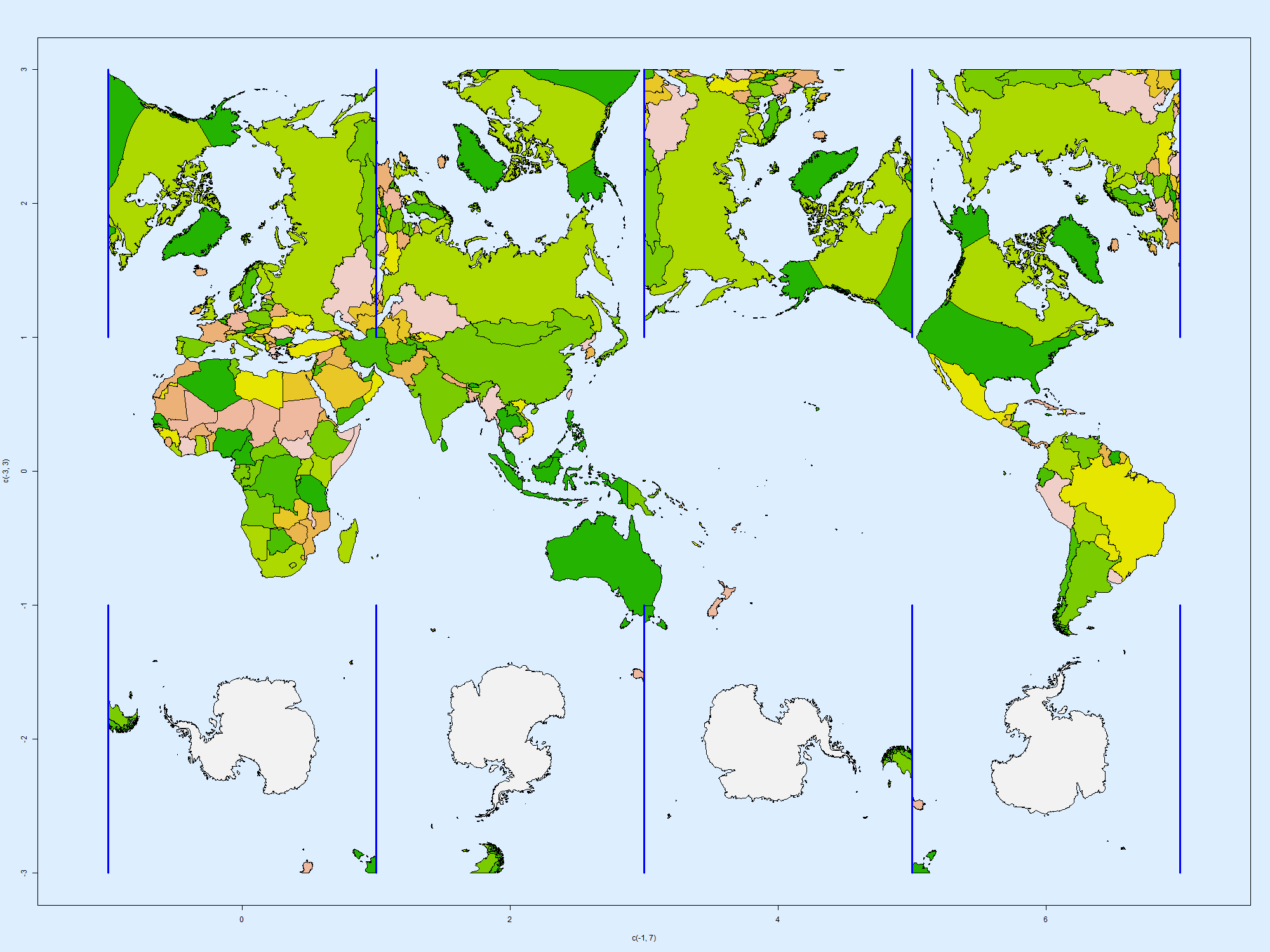
So I wondered how this would work with GISS. It isn't as smooth as UAH, and the 250 km less smooth than 1200km interpolation. So while 18 nodes (6x3) isn't quite enough, 108 nodes (12x9) is pretty good. Here are the plots:


I should add that this is the very simplest grid integration, with no use of enlightened infilling, which would help considerably. The code is here.

Of course, when you look at a statistic over a longer period, even this small noise fades. Here are the GISS trends over 50 years:

1967-2016 trend C/CenFull mesh 108 points 18 points
250km1.6581.7031.754
1200km1.7541.7431.768


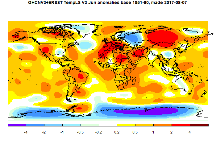
This is a somewhat different problem from my intermittent search for a 60-station subset. There has already been smoothing in gridding. But it shows that the spatial and temporal fluctuations that we focus on in individual maps are much diminished when aggregated over time or space.


Thursday, June 8, 2017

May global temperature unchanged from April

TempLS mesh was virtually unchanged , from 0.722°C to 0.725°C. This follows the smallish rise of 0.06°C in the NCEP/NCAR index, and larger rises in the satellite indices. The May temperature is still warm, in fact, not much less than May 2016 (0.763°C). But it puts 2017 to date now a little below the annual average for 2016.

The main interest is at the poles, where Antarctica was warm, and the Arctic rather cold, which may help retain the ice. There was a band of warmth running from Mongolia to Morocco, and cold in NW Russia.. Here is the map:


Saturday, June 3, 2017

May NCEP/NCAR up 0.06°C

So far in 2017, in the Moyhu NCEP/NCAR index, January to March were very warm, but April was a lot cooler. May recovered a little, rising from 0.34 to 0.4°C, on the 1994-2013 anomaly base. This is still warm by historic standards, ahead of all annual averages before 2016, but it diminishes the likelihood that 2017 will be warmer than 2016.

There were few notable patterns of hot and cold - cold in central Russia and US, but warm in western US, etc. The Arctic was fairly neutral, which may explain the fairly slow melting of the ice..

Update - UAH lower troposphere V6 ;rose considerably, from 0.27°C to 0.45°C in May.